postgibbsf90

How does the program work? This is an interactive program, so just follow the program. name of parameter file?test.par POST-GIBBSF90 2.96 Read 1000 samples from round 10 to 10000 Burn-in? 1000 # in the first run, type 0 for burn-in to include all samples Give n to read every n-th sample? (1 means read all samples) 10 # Type the same number used with a Gibbs sampling program. # samples after burn-in = 9000 Input files: gibbs_samples, fort.99 output files: postgibbs_samples, postout, postmean, postsd "postgibbs_samples" is a file contaning all Gibbs samples for additional post analyses. "postmean" is a file contaning posterior means. "postsd" is a file contaning posterior standard deviations. "postout": ******** Monte Carlo Error by Time Series ******** Pos. eff1 eff2 trt1 trt2 MCE Mean HPD Effective Median Mode Independent Interval (95%) sample size chain size 1 4 4 1 1 1.362E-02 0.9889 0.7788 1.215 70.4 0.9844 0.9861 18 2 4 4 1 2 1.288E-02 1.006 0.777 1.219 84.1 1.006 0.952 18 3 4 4 2 2 1.847E-02 1.66 1.347 1.987 80.3 1.652 1.579 25 4 0 0 1 1 9.530E-03 24.47 24.07 24.84 425.6 24.47 24.53 2 5 0 0 1 2 8.253E-03 11.84 11.54 12.18 395.8 11.83 11.82 2 6 0 0 2 2 1.233E-02 30.1 29.65 30.58 387.8 30.09 29.97 5   ******** Posterior Standard Deviation ******** Pos. eff1 eff2 trt1 trt2 PSD Mean PSD Convergence Autocorrelations Independent Interval (95%) diagnostic lag: 1 10 50 # batches 1 4 4 1 1 0.1144 0.9889 0.7648 1.213 -0.02 0.853 0.188 0.049 50 2 4 4 1 2 0.1182 1.006 0.7742 1.237 -0.11 0.828 0.111 -0.066 50 3 4 4 2 2 0.1656 1.66 1.335 1.984 0.06 0.828 0.108 -0.021 36 4 0 0 1 1 0.1967 24.47 24.09 24.86 -0.01 0.034 0.029 -0.062 450 5 0 0 1 2 0.1643 11.84 11.51 12.16 0.03 0.032 -0.006 -0.016 450 6 0 0 2 2 0.2429 30.1 29.62 30.57 -0.02 0.07 -0.014 0.037 180 "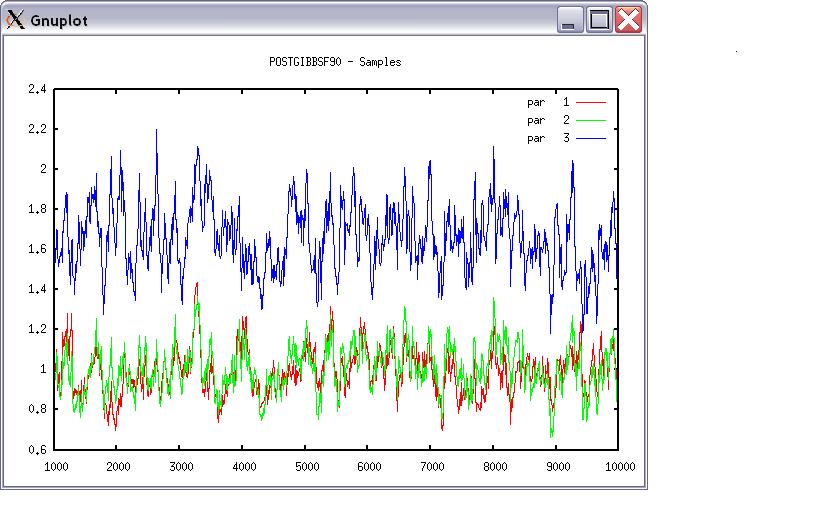Pos.": position of each parameter in the parameter file "eff1" and "eff2": effect number in the parameter file "trt1" and "trt2": trait number in the parameter file "MCE": Monte Carlo Error "Mean": posterior means "HPD interval (95%)": Highest Probability Density "Effective sample size": at least > 10 is recommended. > 30 may be better. "Median": "Mode": when the distribution of the samples is nor normal, there is a difference between "Mode" and "Mean". "Independent chain size": "PSD": Posterior Standard Deviation "PSD interval (95%)": "Convergence diagnostic": ratio between first half and second half of the samples should be < 1.0, but it is not useful because it is < 1.0 most of the time. "Autocorrelations": autocorrelations between two lags. High correlation implies samples are not independent. 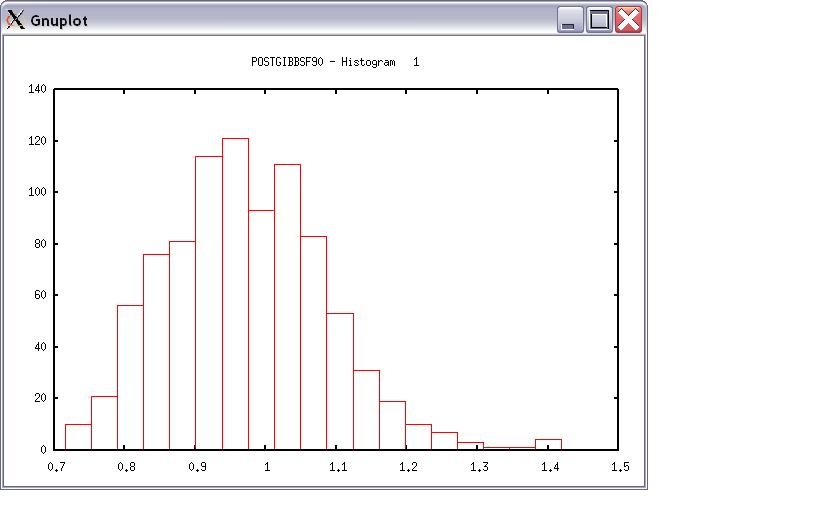"Independent # batches": Choose a graph for samples (= 1) or histogram (= 2); or exit (= 0) 1 positions 1 2 3 # choose from the position numbers 1 through 6 If the graph is stable (not increasing or decreasing), the convergence is met. All samples before that point shoudl be discarded as burn-in. print = 1; other graphs = 2; or stop = 0 2 Choose a graph for samples (= 1) or histogram (= 2); or exit (= 0) 2 Type position and # bins 1 20 The distribution should be usually normal. print = 1; other graphs = 2; or stop = 0 0 *** Log Marginal Density for Bayes Factor *** after 900 burn-in log(p) = -179448.742766031 This value could be used when calculating Bayes Factor or DIC. Need more examples?