POSTGIBBSF90

POSTGIBBSF90 is a post Gibbs analysis program for all Gibbs sampling programs: GIBBSF90, GIBBS1F90, GIBBS2F90, GIBBS3F90, THRGIBBS1F90, and THRGIBBS3F90. This program provides some statistics for “convergence diagnosis” and posterior means and SD.

It calculates posterior means, median, mode, standard deviations, HPD, effective sample size and auto-correlations. It can also display or print the shape of one or more variance components or a histogram of one component.
This is an interactive program, so just follow the program. “gnuplot” is required for drawing graphs.

name of parameter file?test.par

POST-GIBBSF90 2.96

Read 1000 samples from round 10 to 10000

Burn-in?
1000 # in the first run, type 0 for burn-in to include all samples

Give n to read every n-th sample? (1 means read all samples)
10 # Type the same number used with a Gibbs sampling program.

# samples after burn-in = 9000

• input files: gibbs_samples, fort.99
• output files: postgibbs_samples, postout, postmean, postsd
• “postgibbs_samples” is a file contaning all Gibbs samples for additional post analyses.
• “postmean” is a file contaning posterior means.
• “postsd” is a file contaning posterior standard deviations.
• “postout”:

                               ********      Monte Carlo Error by Time Series      ********
Pos.  eff1    eff2    trt1    trt2         MCE      Mean        HPD        Effective  Median   Mode  Independent
				                           Interval (95%)  sample size               chain size
1 	4 	4 	1 	1 	1.362E-02  0.9889  0.7788  1.215     70.4     0.9844  0.9861      18
2 	4 	4 	1 	2 	1.288E-02  1.006   0.777   1.219     84.1     1.006   0.952       18
3 	4 	4 	2 	2 	1.847E-02  1.66    1.347   1.987     80.3     1.652   1.579       25
4 	0 	0 	1 	1 	9.530E-03  24.47   24.07   24.84    425.6     24.47   24.53        2
5 	0 	0 	1 	2 	8.253E-03  11.84   11.54   12.18    395.8     11.83   11.82        2
6 	0 	0 	2 	2 	1.233E-02  30.1    29.65   30.58    387.8     30.09   29.97        5

				********      Posterior Standard Deviation      ********
Pos.  eff1    eff2    trt1    trt2        PSD       Mean       PSD         Convergence     Auto-correlations   Independent
                                                           Interval (95%)  diagnostic  lag: 1     10      50   # batches
1 	4 	4 	1 	1 	0.1144    0.9889   0.7648  1.213     -0.02      0.853 	0.188   0.049     50
2 	4 	4 	1 	2 	0.1182 	  1.006    0.7742  1.237     -0.11      0.828 	0.111  -0.066     50
3 	4 	4 	2 	2 	0.1656 	  1.66     1.335   1.984      0.06      0.828 	0.108  -0.021     36
4 	0 	0 	1 	1 	0.1967 	  24.47    24.09   24.86     -0.01      0.034 	0.029  -0.062    450
5 	0 	0 	1 	2 	0.1643 	  11.84    11.51   12.16      0.03      0.032  -0.006  -0.016    450
6 	0 	0 	2 	2 	0.2429 	  30.1 	   29.62   30.57     -0.02      0.07   -0.014   0.037    180

• “Pos.”: position of each parameter in the parameter file
• “eff1” and “eff2”: effect number in the parameter file
• “trt1” and “trt2”: trait number in the parameter file
• “MCE”: Monte Carlo Error
• “Mean”: posterior means
• “HPD interval (95%)”: Highest Probability Density
• “Effective sample size”: at least > 10 is recommended. > 30 may be better.
• “Median”:
• “Mode”: when the distribution of the samples is nor normal, there is a difference between “Mode” and “Mean”.
• “Independent chain size”:
• “PSD”: Posterior Standard Deviation
• “PSD interval (95%)”:
• “Convergence diagnostic”: ratio between first half and second half of the samples should be < 1.0, but it is not useful because it is < 1.0 most of the time.
• “Autocorrelations”: autocorrelations between two lags. High correlation implies samples are not independent.
• “Independent # batches”:

Hint: when eff1, eff2, trt1, trt2 are all -1, the values presented are for thresholds (if THRGIBBSXF90 is used).

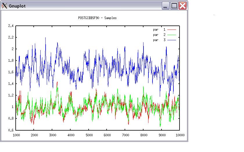
Choose a graph for samples (= 1) or histogram (= 2); or exit (= 0)
1

positions

1 2 3 # choose from the position numbers 1 through 6

If the graph is stable (not increasing or decreasing), the convergence is met.
All samples before that point should be discarded as burn-in.

print = 1; other graphs = 2; or stop = 0
2

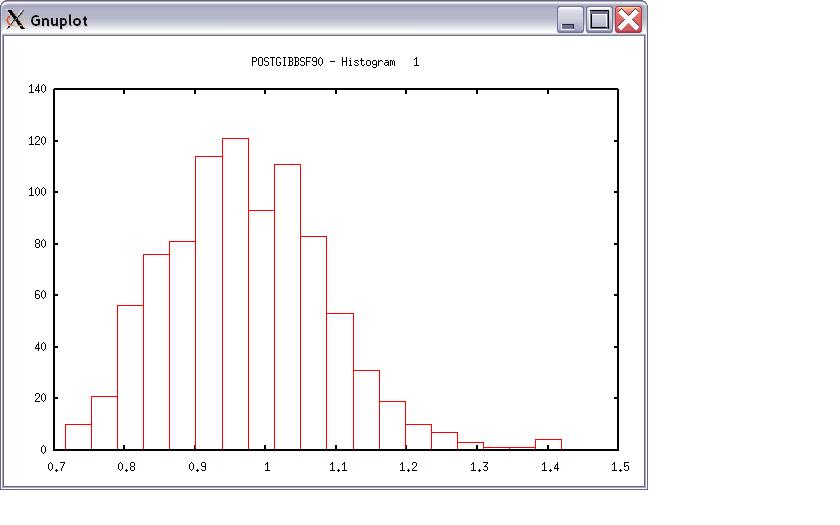
Choose a graph for samples (= 1) or histogram (= 2); or exit (= 0)
2

Type position and # bins
1 20

The distribution should be usually normal.

print = 1; other graphs = 2; or stop = 0
0

*** Log Marginal Density for Bayes Factor ***
after 900 burn-in
log(p) = -179448.742766031

• This value could be used when calculating Bayes Factor or DIC.

OPTION se_covar_function <label> <function>

This option calculate post Gibbs statistics for function of (co)variances (heritability, correlation, etc).

<label>
A name for a particular function (e.g., P1 for phenotypic variance of trait 1, H2_1 for heritability for trait 1, rg12 for genetic correlation between traits 1 and 2, …).

<function>
A equation to calculate a function of (co)variances. All terms of the function should be written with no spaces between them.

Each term of the function corresponds to (co)variance elements and could include any random effects (G) and residual (R) (co)variances.

Notation is with reference to the effect number and the trait number (G_eff1_eff2_trt1_trt2) that indicate the element of the (co)variance matrix for random effect eff1 and eff2 and trt1 and trt2,
where eff1 and eff2 are effect numbers 1 and 2, and trt1 and trt2 are trait numbers 1 and 2.
R_trt1_trt1 indicates the element of the residual (co)variance matrix for traits 1 and 2.

Several functions could be added, with one OPTION line per function.

Examples:

OPTION se_covar_function P G_2_2_1_1+G_2_3_1_1+G_3_3_1_1+G_4_4_1_1+R_1_1

OPTION se_covar_function H2d G_2_2_1_1/(G_2_2_1_1+G_2_3_1_1+G_3_3_1_1+G_4_4_1_1+R_1_1)

OPTION se_covar_function H2t (G_2_2_1_1+1.5*G_2_3_1_1+0.5*G_3_3_1_1)/(G_2_2_1_1+G_2_3_1_1+G_3_3_1_1+G_4_4_1_1+R_1_1)

OPTION se_covar_function rg12 G_2_2_1_2/(G_2_2_1_1*G_2_2_2_2)**0.5

The first function calculates the total variance for a maternal model with permanent maternal effect, where 2 and 3 are the effect number for the direct and maternal additive genetic effects respectively, and 4 is the effect number for the maternal permanent random effect.

The second function calculates the heritability for the direct component.

The third function the total heritability.

The fourth function calculates the genetic correlation between traits 1 and 2 for the direct genetic effect (effect number 2)